Building Simple Linear Regression from Scratch: No Libraries, Just Math

Welcome back to the lab. 🧪

Today, I will show you how Simple Linear Regression models work under the hood and how you can build one from scratch without relying on “black box” libraries like Scikit-Learn.

1. Logic First: Understanding Correlation

Before we dive into equations, we must understand the behavior of data. Linear Regression is essentially an attempt to quantify the relationship between two variables.

Imagine you want to analyze the link between Years of Experience and Salary. Intuitively, we expect that as experience grows, the salary increases. In statistics, we call this a Positive Correlation. The variables move in the same direction.

Now, let’s consider a different scenario: The relationship between Parental Anger Levels and Allowed Gaming Hours. As your mother gets angrier, your allowed gaming time likely drops to zero. Here, one value increases while the other decreases. This is a Negative Correlation.

Finally, if you were to plot the Current Time of Day against your Bank Account Balance, you would likely find no meaningful pattern. The time of day does not dictate your wealth. This is a case of Zero Correlation.

In Linear Regression, our goal is to find a mathematical line that best describes these positive or negative relationships so we can predict future outcomes.

2. The Math: Investigating the “Best Fit”

We agreed that we want a line. But there are infinite lines we could draw. How do we prove, mathematically, that one line is better than all others?

We treat this as an optimization problem.

Step 1: Defining the Enemy (The Error)

For every single data point, our line will likely be wrong. The distance between the real point and our line is called the Residual (Error).

We want the total error to be as low as possible. But we can’t just add them up, because negative errors (points below the line) would cancel out positive errors (points above the line).

To solve this, we square the errors. This turns all negatives into positives and heavily penalizes large mistakes. This gives us our Cost Function (S):

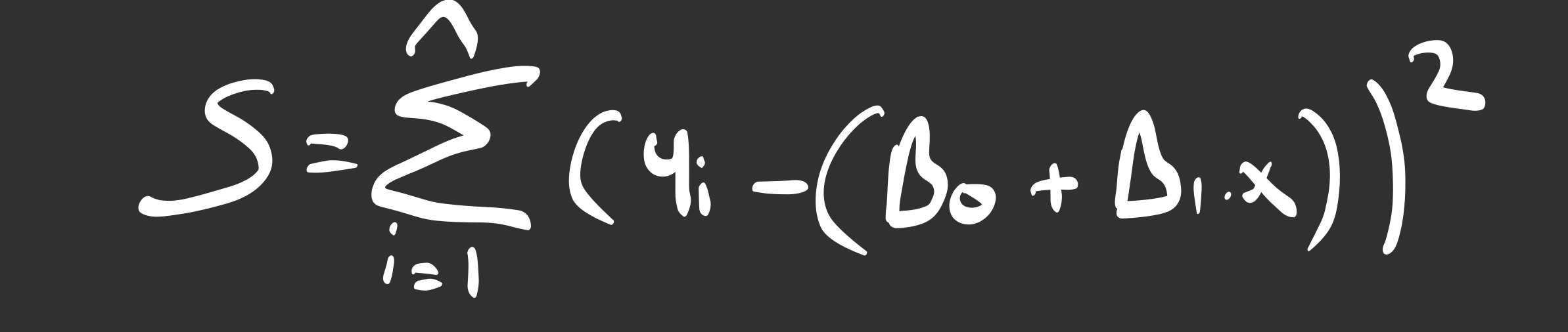
Our Mission: Find the values of Beta 0 and Beta 1 that make S as small as possible. Imagine this function as a valley; we want to find the deepest point.

Step 2: The Weapon (Calculus)

In Calculus, the bottom of a curve (the minimum point) is where the slope is zero.

So, we take the Partial Derivative of our error function with respect to both Betas and set them to zero.

Derivation A: Finding the Intercept (Beta 0)

Imagine moving the line up and down without changing its angle. Where should it stop?

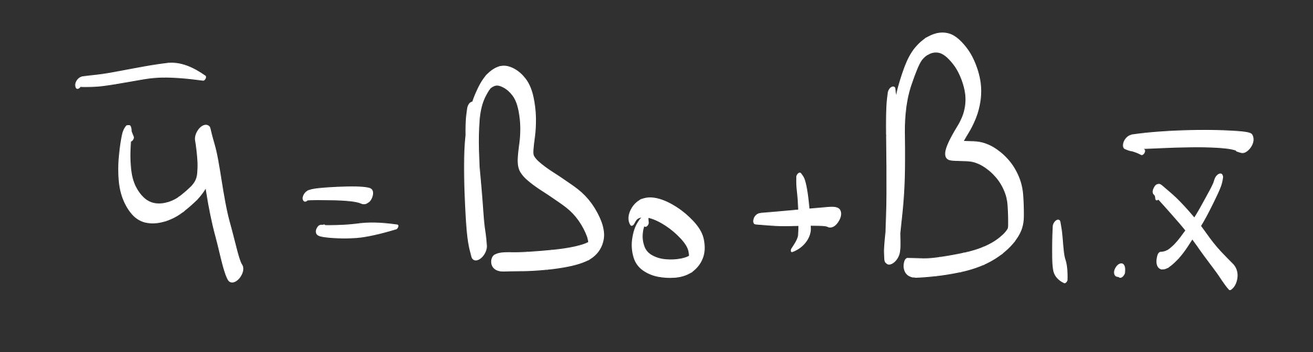
We take the derivative with respect to Beta 0:

When we simplify this, the math reveals a simple truth: The best regression line must pass through the average of x and the average of y. It is the line’s center of gravity.

Derivation B: Finding the Slope (Beta 1)

Now, imagine rotating the line around that center point. What is the perfect angle?

We take the derivative with respect to Beta 1. This time, the Chain Rule pulls out an ‘x’ term because the slope is multiplied by x.

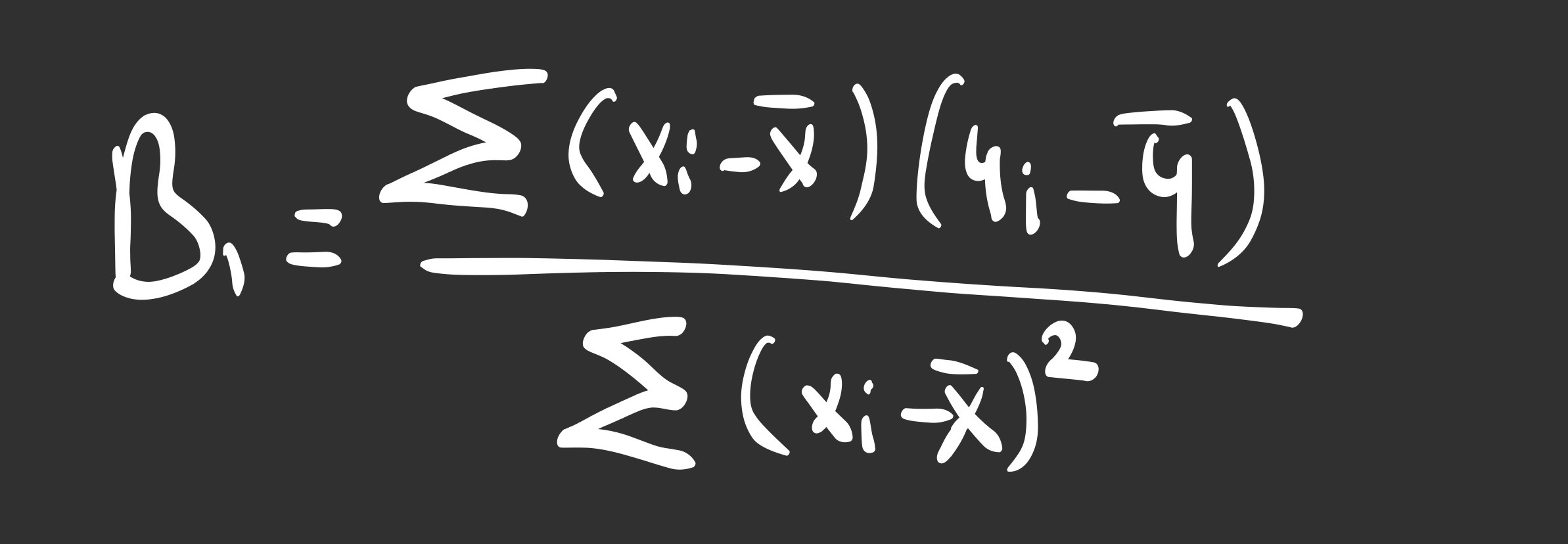
After rearranging the terms and substituting our equation for Beta 0, we arrive at the “Golden Formula”:

Conclusion of the Math

Look closely at that fraction. Calculating the slope isn’t magic.

• The Numerator is the Covariance. It measures how much X and Y move together.
• The Denominator is the Variance. It measures how much X moves by itself.

It is simply asking: “For every unit of variation in X, how much of it corresponds to a variation in Y?”

Implementation: Turning Math into Machine Learning

Now that we have derived the formulas for the slope ($\beta_1$) and the intercept ($\beta_0$), it is time to build the engine.

I have structured the code into two distinct parts:

1. The Engine (The Class): Where the logic and “memory” live.
2. The Driver (Execution): Where we feed data and test the model.

Part 1: The Engine (The Class Logic)

We use Python’s Object-Oriented Programming (OOP) to create a blueprint. This allows our model to have “state”—meaning it can learn something in one step and remember it for the next.

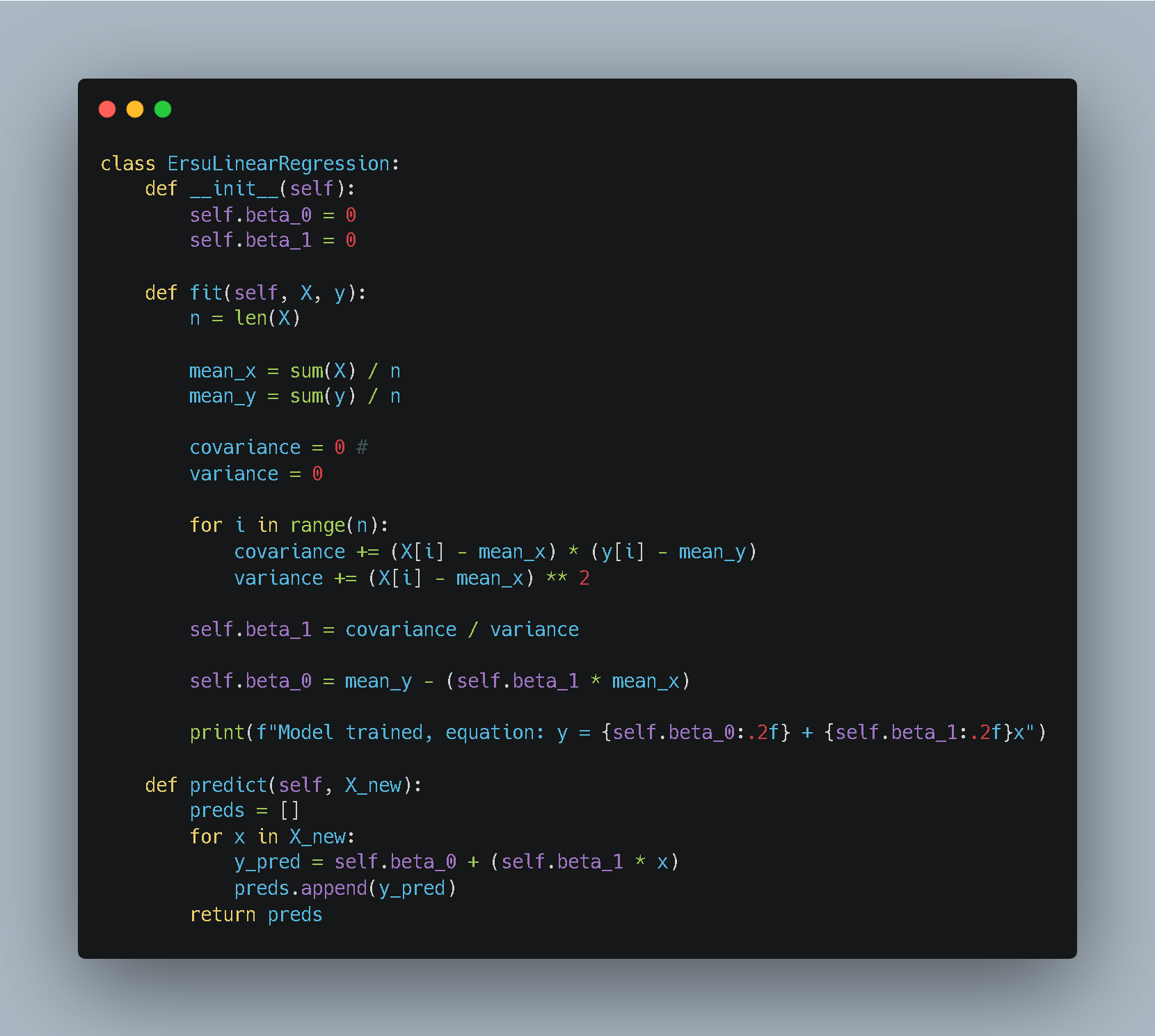
Breaking Down the Engine:

• __init__: This is the constructor. It initializes our slope and intercept to zero. The model starts with a “blank mind.”
• fit(X, y): This is the training phase. It takes the raw data, applies the Least Squares formulas we derived, and saves the results into self.beta_0 and self.beta_1. It doesn’t return a value; it simply updates its internal memory.
• predict(X_new): This is the deployment phase. It takes new, unseen inputs and uses the learned coefficients to calculate predictions using the line equation $y = \beta_0 + \beta_1 x$.

---

Part 2: The Driver (Training & Prediction)

A car engine is useless without fuel and a driver. In this section, we create some dummy data, instantiate our model, and take it for a test drive.

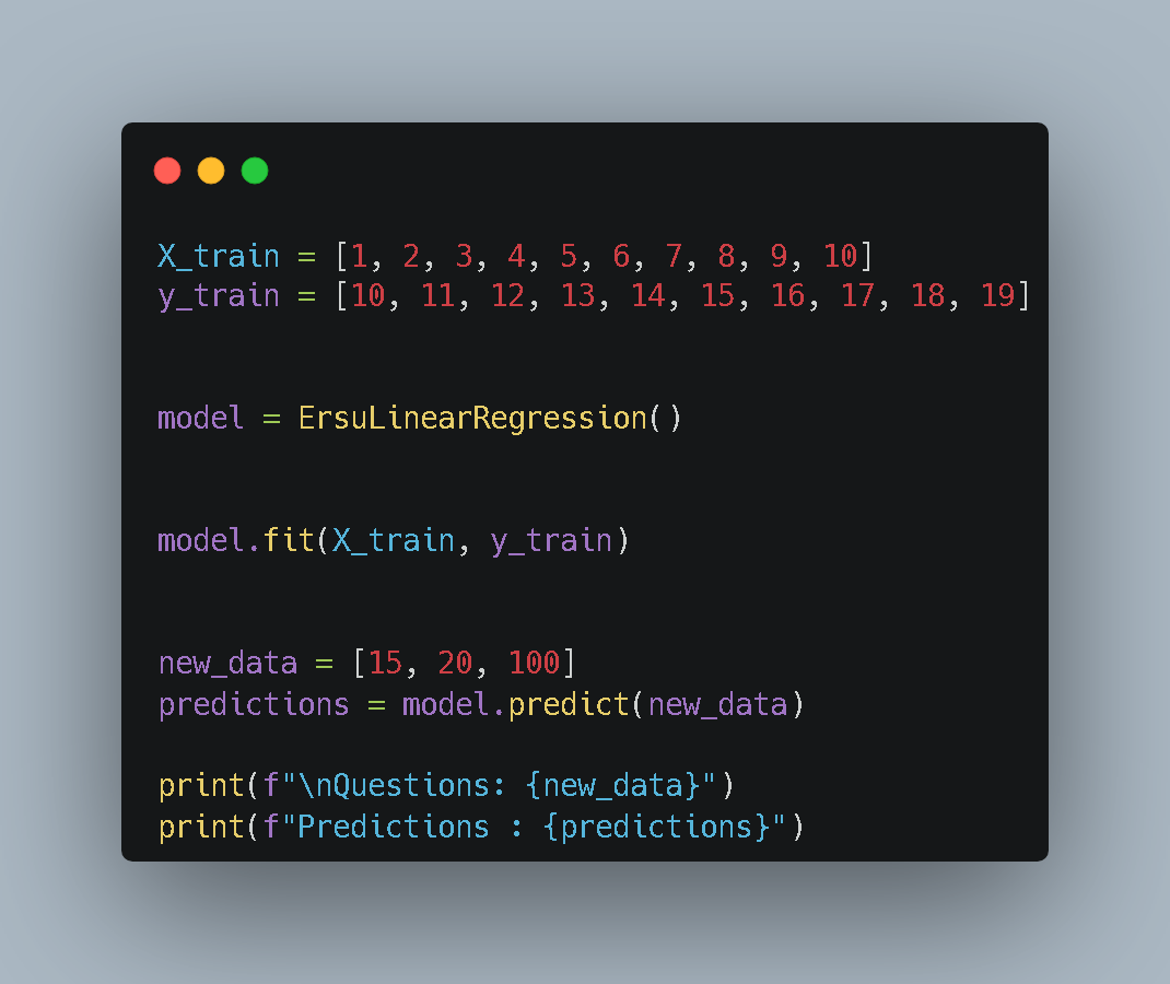
The Workflow:

1. Data Preparation: We define simple lists for X (input) and y (target).
2. Instantiation: model = ErsuLinearRegression() creates a new instance of our class.
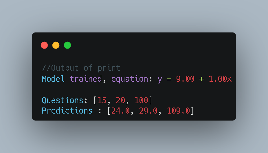
3. Training: We call .fit(X, y). At this moment, the math happens, and the model “learns” the relationship.
4. Prediction: We ask the model, “If X is 15, what is y?” and print the result to verify our logic.

---

Conclusion: Closing the Notebook

What have we proven in the lab today? We stripped the chassis off the “Machine Learning” car and found that there is no magic engine inside. It is just pure, elegant mechanics.

We proved that Linear Regression is nothing more than a specific ratio: quantifying how much two things move together (Covariance) versus how much they move apart (Variance).

However, our current model has a flaw.

It views the world through a single lens (one x). But reality is rarely univariate. A house price isn’t just about size; it’s about location, age, and room count. Predicting real-world phenomena with a simple line is like trying to solve a puzzle with missing pieces.

Next time in the Lab: We are going to upgrade our engine. We will leave the simple algebra behind and enter the world of Linear Algebra. We will build a Multiple Linear Regression model using Matrices, allowing us to predict outcomes based on infinite variables simultaneously.

Until then, keep experimenting.