Mastering Gradient Descent: The Art of Feature vs. Target Scaling

Welcome back to the lab. 🧪

Gradient Descent is the backbone of modern machine learning optimization. However, as I discovered in this latest experiment, its performance is incredibly sensitive to the scale of your data.

In my previous projects, I relied on libraries to handle the heavy lifting. This time, I built a Multiple Linear Regression (MLR) model from scratch using batch Gradient Descent to answer a specific question: Should we scale just the inputs, or the targets as well?

Here is my log of the experiment.

1. The Engine: Building the Regressor

Before running the tests, I implemented the math manually. The prediction function $\hat{y}$ for a given input vector is defined as:

$$ \hat{y} = w_{1}x_{1} + w_{2}x_{2} + ... + w_{n}x_{n} + b $$

To train this, I used the Mean Squared Error (MSE) cost function. It’s perfect for Gradient Descent because it is convex and differentiable, meaning we can easily find the bottom of the “error valley”.

$$ J(w,b) = \frac{1}{n}\sum_{i=1}^{n}(y_{i}-\hat{y}_{i})^{2} $$

The weights were updated iteratively using the gradients:

$$ w_{j} := w_{j} - \alpha\frac{1}{n}\sum_{i=1}^{n}(\hat{y}_{i}-y_{i})x_{ij} $$

2. The Setup

I used a student performance dataset ($n=10,000$). To evaluate the results fairly, I looked at the MSE for the loss, but I also calculated the Mean Absolute Percentage Error (MAPE) to get a percentage-based accuracy score.

I ran three distinct experiments to see how scaling affected convergence.

3. Experiment I: The “Hybrid” Approach (Winner) 🏆

Configuration:

• Inputs (X): Normalized to a standard range.
• Targets (y): Left in their natural scale (0-100 exam scores).

The Result: This configuration was the clear winner. The model converged within 2,000 epochs with a MAPE of 3.73%.

As you can see in the plot below, the predictions (blue dots) tightly follow the ideal red diagonal line, proving the model learned the distribution perfectly.

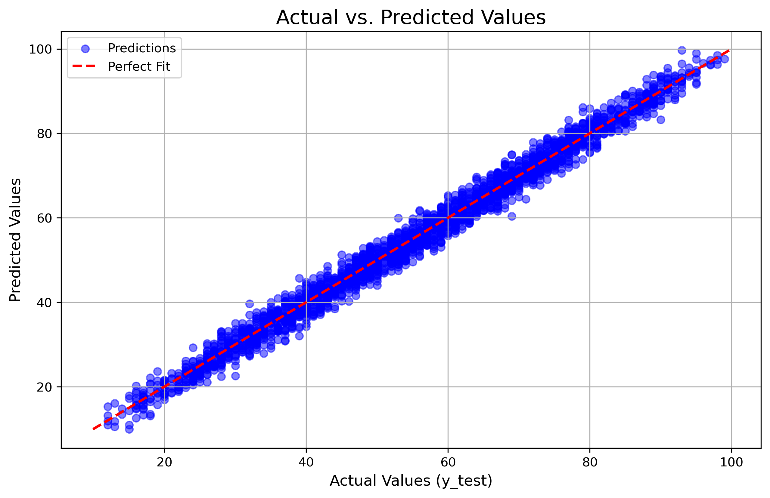(Figure 1: High accuracy fit with $R^2 \approx 0.99$)

4. Experiment II: The “Raw Data” Chaos

Configuration:

• Inputs (X): Unnormalized (Raw).
• Targets (y): Unnormalized (Raw).

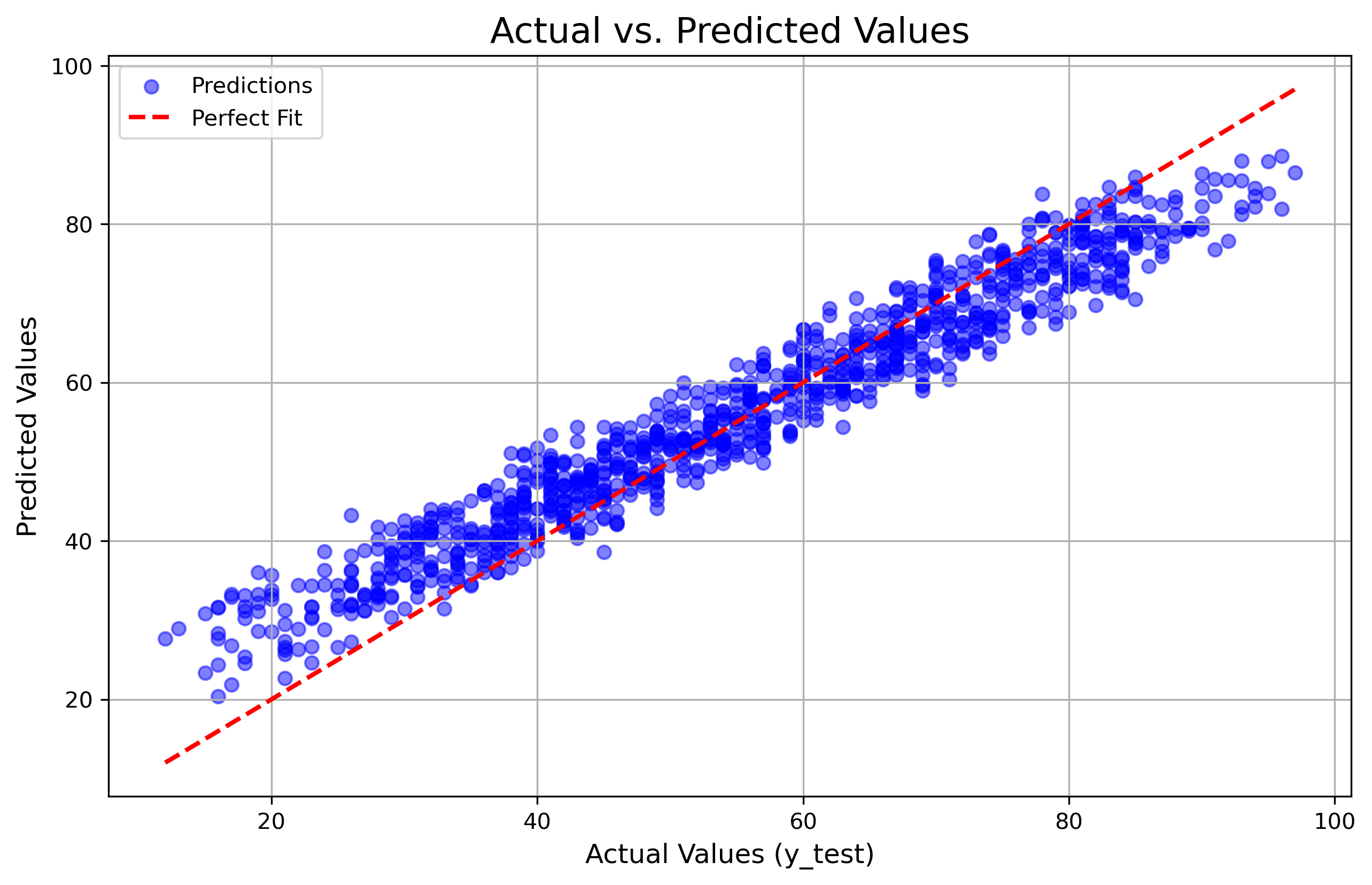
The Result: This was a disaster. The unnormalized inputs created an elongated loss landscape. When I used a standard learning rate ($\alpha=0.01$), I hit an Overflow error—Exploding Gradients.

I had to reduce the learning rate to a tiny $0.0001$ just to get it to run, and even then, the performance degraded significantly (MAPE 11.52%). The scatter plot showed much higher variance (noise) compared to Experiment I.

5. Experiment III: The “Over-Normalization” Trap

Configuration:

• Inputs (X): Normalized [0, 1].
• Targets (y): Normalized [0, 1].

The Result: This was the most surprising finding. I assumed scaling everything would be better, but the model stopped learning entirely.

This led to the Vanishing Gradient problem. Because the target values were so small (< 1), the calculated gradients approached zero. The weights didn’t update significantly, and the model got stuck predicting the mean of the dataset for every single student.

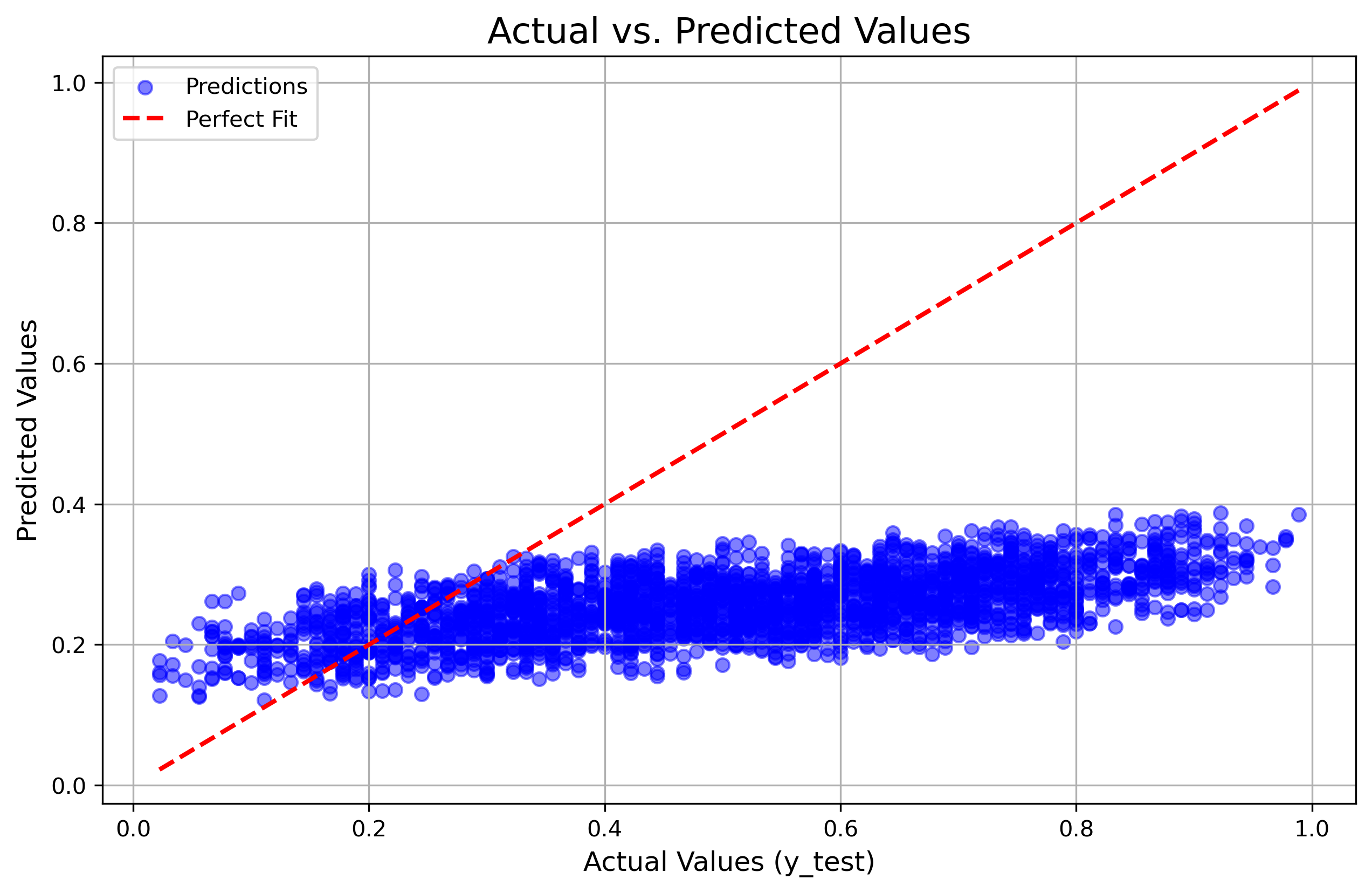(Figure 3: The “Flatline.” The model fails to learn the slope entirely.)

Conclusion

This experiment provided empirical evidence of an asymmetry in Gradient Descent.

1. Scale your inputs: It is non-negotiable for numerical stability and preventing exploding gradients.
2. Don’t scale your targets (usually): For regression tasks with bounded outputs, scaling targets to [0, 1] can compress gradients too much, trapping the model.

The optimal configuration is a hybrid one: Normalized Inputs + Natural Scale Targets. This achieved the best balance of stability and precision (3.73% error).

Next time, I’ll be looking into how different weight initialization strategies might help solve some of these issues from the start!